
|
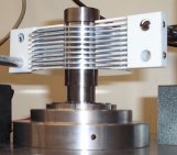
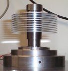
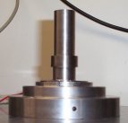
| Figure 16 : AEM Test Setup (Probe and Adapter with Disk Stack and Fingers) |
AEM Measurements
We use the Lion Precision Spindle Error Analyzer software to make the asynchronous error motion measurements. We use the same Lion capacitance probes and drivers as for the dynamic stiffness tests, but this time we use the probes on the HI range setting, since the magnitude of the AEM is much smaller and we need more accurate readings.The Lion software automatically subtracts out the synchronous error motion when making the asynchronous error measurements, which should minimize the effects of any imbalance in the target. The software also triggers its measurements from the encoder pulses, so that should minimize the corrupting effects of the velocity modulation.The measurements are on such a small scale, however, that the condition of the probe target is very critical for accuracy. The target mounted on the bearing spindle needs to be as round and centered and have the best surface finish possible to sense very delicate motions of the rotor.
For these tests we use the disk stack adapter attachment. Again, the axial location of the measurements is a very important variable, so we chose a distance of one inch from the top of the bolt heads holding the adapter onto the rotor. This spot gives us enough room to leave the probe in place and put the stack of disks and spacers on the adapter. Since the probe is closer to the center of the bearing than the disks, the AEM measurements will be best-case readings. We would have preferred to have the probe in a location that would have given us worst-case readings so we could estimate the motion of the top disk, but we found that difficult to pull off procedurally.
|
|
| Figure 16 : AEM Test Setup (Probe and Adapter with Disk Stack and Fingers) |
The picture above shows a typical disk stack setup for making the AEM measurements.We take the measurements over a range of spindle speeds with disks and fingers in place, with only the disks and no fingers, and then without disks or fingers.We use nine disks in the disk stack since that is the maximum number of disks that the model of the disk stack adapter could hold.
The Lion Spindle Error Analyzer software measures and computes the AEM measurement by taking readings over 25 spindle revolutions. The software continues to take measurements every 25 revolutions or so and displays the latest AEM value. The AEM values vary slightly from measurement to measurement, so to find a representative value we sample 20 AEM measurements in a row and take the mean.
Velocity Modulation Measurements
For the velocity modulation measurements we again use the disk stack adapters just as we did for the AEM measurements. Again we take the measurements over a range of bearing speeds with disks and fingers in place, with only the disks and no fingers, and then without disks or fingers.
|
|
|
| Fingers | Disks | Bare |
| Table 1: Velocity Modulation Test Setups | ||
This time, though, instead of using a capacitance probe to look at the rotor runout, we use a modulation domain analyzer to look at the output of the encoder to figure out how the velocity of the spindle changes with time.
|
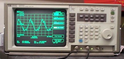
| Figure 17: Modulation Domain Analyzer HP 53310A |
The modulation domain analyzer has two inputs, the frequency signal input and an optional trigger. The modulation analyzer measures how the frequency of the input signal changes with time.It can display the information in two ways: 1) Cartesian coordinates with frequency on the dependent axis versus time on the independent and 2) a histogram of the distribution of measured frequencies. The analyzer computes the mean (m) and standard deviation (s) of the distribution of frequencies. The units of these numbers are hertz and we use them to compute the percent velocity error.We approximate the range of the distribution as 6s, so the total variation about the mean is plus or minus 3s.
|
|
| Equation 5: Velocity Modulation Percent Error |
We examine the standard encoder output for the short-term intra-revolution velocity modulation and the index pulse from the encoder for the long-term inter-revolution velocity modulation. As mentioned in the background, the frequency variance depends heavily on the time scale that the frequency is measured over. Somewhat arbitrarily we chose to examine the intra-revolution velocity error over 3 revolutions and the inter-revolution velocity error over 1000 revolutions.So at each RPM, we had to set the modulation analyzer time scale so that the range corresponded to the number of revolutions we wanted to measure over.The standard deviation also depends on the number of samples, so we fixed the number of samples per test at 20,000.The intra-revolution measurements are somewhat flawed in that they depend on the encoder count, but all of the encoders used in these tests had 1024 count encoders, so at least they were consistent. We did not include the Brand A spindles in the velocity modulation tests since they use encoders with 512 counts and since we had to use another controller to spin them.
Test Results
The first step of the testing was to design setups that yielded repeatable results.There were many sources of potential corruption and they all needed to be controlled or at least minimized. The air flow and motor current measurements were valuable for diagnosing system problems.We found that some of the most influential variables were the air supply pressure, the electrical ground paths throughout the system, the bearing support structure, and the probe holders. Some of the bearings with very high flow caused the air supply pressure to fluctuate, so we added air tanks to act as air supply capacitors.This allowed the spindles to all run steadily at their rated air supply pressures. Good electrical grounding in the system was crucial for reliable capacitance probe readings.It was especially important that the rotors stay properly grounded. At high bearing speeds the imbalances used in the dynamic stiffness tests created very large forces throughout the entire support structure.Everything in the support structure had to be as rigid and held as securely as possible to minimize unwanted motion.Since we were trying to measure the motion of the rotor with respect to the stator, the probe holders needed to be as rigid and as lightweight as possible to minimize the amount of motion between the probe tip and the stator.Any probe holder has natural frequencies and resonant modes, however, so the transfer function between stator and probe tip might always affect the frequency response tests, depending on the frequency ranges.
Dynamic Stiffness
The first relationship between variables that we wanted to check with the dynamic stiffness tests was how the dynamic stiffness varied with the radial displacement of the rotor axis. We assumed that the dynamic stiffness might both be a function of bearing RPM and the radial displacement of the rotor axis. This could mean potentially having to examine the data three-dimensionally, with dynamic stiffness as the dependent variable and both the RPM and the radial displacement as independent variables.Since it is more convenient to examine the data two-dimensionally, we decided to first check how the dynamic stiffness varied with radial displacement at a constant RPM value, on the chance that the variation would be small and we could assume it to be negligible.

|
| Figure 18 : Dynamic Stiffness vs. Radial Displacement at 10,000 RPM |
The plot above shows how the dynamic stiffness varies with radial displacement for one of the bearings at 10,000 RPM. Each data point represents a unique imbalance introduced into the stiffness adapter.The dynamic stiffness seemed to remain very constant with radial displacement, so for the rest of the dynamic stiffness tests we only measured the dynamic stiffness with a single imbalance magnitude (0.3 gram-inches). As an additional check, we also examined how the direction of the displacement changed with the various imbalance amounts at 10,000 RPM.Assuming that the phase angle remains constant at a given rotational velocity (not necessarily true if the air film properties change with rotor radial displacement), the displacement should always be in the same radial direction, regardless of the amount of imbalance.

|
| Figure 19 : Rotor Axis Displacement Polar Plot |
The plot above is a polar plot of the rotor axis and how it moves with the varying magnitudes of centrifugal force acting on the rotor. Except for one outlying point, the rotor axis seems to move repeatedly in the same radial direction. The point closest to the origin is the location of the adapter axis when the adapter is balanced. The points move away from the origin as the imbalance, and therefore the centrifugal force, increases. Note that the balanced location does not coincide with the origin. The distance between the balanced location and the origin is the amount that the stiffness adapter axis is off center from the rotor axis.
The next step in the stiffness testing was to perform the stiffness tests for each of the eight bearings over a range of speeds.

|
| Figure 20 : Dynamic Stiffness vs. RPM for All Air Bearings Tested |
The plot above shows the results of the dynamic stiffness tests for the bearings.The dynamic stiffness is plotted on the dependent axis versus the RPM on the independent axis.Each color represents one type of bearing (4 types in total), there were two bearings of each type (8 bearings), and each bearing was tested twice (16 tests in total).Brand A measured between 10,000 and 15,000 lb/in and the Seagull standard Biconic measured between 15,000 and 20,000 lb/in. The two Brand D bearings showed very different results. The one with the higher stiffness had almost twice the air flow of the one with the lower stiffness, so perhaps they were built differently or one was damaged in some way.The new Seagull Hi-Capacity Biconic air bearing spindle was designed for high stiffness and high speed and the results show this to indeed be true.The stiffness of the Hi-Capacity Biconic was over twice that of the standard Biconic and was measured all the way up to 28,000 RPM, limited only by the amplifier supply voltage.We had to limit the maximum speed of the other bearings because we either reached their maximum rated RPM or because the rotor displacement was too large to measure under the load.
AEM
We found that the AEM measurements are very sensitive to external conditions.Any vibrations transmitted through the foundation from the outside world showed up in tests and increased AEM.With our setup, we were not able to measure any significant differences in AEM magnitude between the bearings. They all measured comparably with similar external conditions to the accuracy of our experimental setup. We were, however, able to measure significant differences in the AEM with changes in the disk stack for all of the bearings.

|
| Figure 21 : Typical AEM vs. RPM Test Results |
The chart above shows typical AEM results for the bearings. With just the disk stack mounted on the rotor, all of the bearings showed around half a micro-inch AEM. In reality this number is probably somewhat lower due to probe noise and external vibrations.The probe noise was measured around 0.27 micro-inches. The numbers shown in the chart are the raw measurements without any sort of noise correction.The AEM increased dramatically when the disks were placed on the adapter and seemed to increase linearly or perhaps quadratically with RPM. When the fingers were placed in the disk stack, the AEM reduced significantly.This suggests that the puffing phenomenon in the air layers between the disks in the stack is a major source of disturbance motion in the rotors. Another observation we made was that the motor current doubled with the disks on the adapter.The motor current increased by another 20% with the fingers in the stack. This extra current can create thermal issues in the amplifier and the bearing, so Seagull's Hi-Capacity air bearing spindle uses an ironless-coreless low induction motor, to reduce the motor current consumption.
Velocity Modulation
Intra-Revolution
We found that the frequency modulation of the typical encoder output was so large that we were unable to distinguish the velocity variation from the encoder distortion for the short-term intra-revolution tests.The following table shows our results for these tests, both with the special Low-Modulation (LM) encoder with the centerable encoder disk used on the Hi-Capacity Biconics and the typical encoders used on the others.
|
Encoder Frequency Modulation Versus Time |
|

|

|
|
Typical Encoder |
Adjusted LM Encoder 170.666kHz+/-36Hz +/- 0.02% error |
|
Ideally the graphs above should be straight horizontal lines.For a given RPM, the encoder pulse output frequency should be a single constant value.The typical encoder output varies like a sine wave, though, because the optical disk is off center. Within the revolution, some of the encoder pulses are too fast and others are too slow. The optical disk on the LM encoder can be centered, however, giving a much more constant frequency output. The frequency modulation of the LM encoder is over 8 times less than that of a typical unadjusted encoder. |
|
| Table 2: Encoder Frequency Modulation vs. Time | |
| Frequency Histogram | |

|

|
|
These two graphs show the distribution of the frequency output from both encoders. The unadjusted encoder has a large frequency range with most of the values jumping back and forth between the two frequency extremes.A double-peaked histogram is typical of a sinusoidal variation.The frequency distribution of the LM encoder, however, is very tight and centered about the correct value, with most of the variation due to random noise. |
|
| Table 3 : Encoder Frequency Modulation Histograms | |
Note: All of the images from the modulation domain analyzer are shown on equal scales for comparison.
Inter-Revolution
The long-term inter-revolution velocity modulation tests were not affected by the encoder modulation, since only the index pulse from the encoder was examined.The controller used for these experiments calculates the rotational velocity by averaging the encoder output over several bearing revolutions, so it is effectively blind to the encoder modulation within each revolution.This means that the encoder modulation does not show up as velocity error, but unfortunately this also means that the controller cannot correct short-term velocity error either.The rotor essentially coasts under open loop control over the time it takes the encoder to determine the rotational velocity. Ideally controllers should be able to make short-term corrections in the velocity error, but with such a tight control loop, the encoder modulation will affect velocity error unless a low modulation encoder is used.
As with the AEM experiments, we were unable to measure much variation in the long-term velocity modulation between the spindles. Also, the velocity modulation is very controller dependent, so it is not practical to compare the bearings in this test since the controller we used was optimized for the motors in the Seagull air bearing spindles. Again, though, just as with the AEM experiments, we were able to measure a very significant difference when the disks were placed on the adapter for all of the bearings.

|
| Figure 22 : Typical Inter-Revolution Velocity Modulation vs. RPM Test Results |
With the adapter alone, the inter-revolution velocity error was well under 0.001%.With the disks on the adapter, however, the velocity modulation increased to over 0.005% for all of the bearings tested and increased with RPM. With the fingers installed, though, the velocity modulation decreased to almost the same level as just the bare adapter. Again the puffing phenomenon seems to be having a very significant influence on the spindle performance. The histograms of the velocity distribution are also very telling as to the effect of the disks and the fingers.

|

|

|
| Disks | Fingers | Bare |
| Table 4: Velocity Distribution Histograms | ||
The histograms are screen shots from the modulation domain analyzer.All of the histograms are shown on the same scale for proper comparison. The bare adapter shows almost no variation in the velocity and most of the measurements occur at the correct velocity value. When the disks were placed on the adapter, on the other hand, the velocity measurements show a large amount of random variation. The distribution is Gaussian, as typical for random phenomenon, and wide showing that the values occur over a broad range. With the fingers in the disk stack, however, the distribution returns to almost as narrow of a peak as the bare adapter alone.
Conclusion
The three parameters tested in these experiments seem to be very valuable for quantitatively measuring the performance of air bearings and their support systems.We found Seagull's new Hi-Capacity Biconic air bearing to be over twice as stiff as Seagull's standard Biconic air bearing, which itself had higher stiffness than the competitor bearings we tested. We were not able to measure any significant difference in the AEM and the velocity modulation between the spindles, but we did find that a stack of disks mounted on the rotor greatly reduces spindle performance and that fingers placed in between the disks in the stack almost negates the negative effects of the disks. We found that we were not able to measure the short-term velocity modulation of the spindles because the frequency modulation of a typical encoder is too large.We were, however, able to reduce the encoder modulation almost entirely with Seagull's new low modulation encoder, which will be critical for control loop improvements in the future. The dynamic stiffness tests were valuable for measuring bearing stiffness, but they also have potential to provide a great deal of information as to the frequency response characteristics of the air bearing spindle and the surrounding support structure. Detailed frequency response tests would indicate natural frequencies and resonant modes in the system and give clues about the relationship between variables in the system and the approximate magnitude of various system parameters.We here at Seagull intend to continue to improve the performance of our spindles and the support system using these tests, and improvements of these tests, as a guide.We encourage others to try similar experiments and to work to refine them so the entire industry can benefit from improvement through testing and experimentation.