|
|
|
Measuring Air Bearing Spindle Performance
Peter Polidoro
Dec 2001
|
|
Abstract
In this paper we measure the performance of air bearing spindles with three quantities: the dynamic stiffness, the asynchronous error motion (AEM), and the rotational velocity modulation. The dynamic stiffness is a measure of how well the bearing resists shifts in the rotor axis due to forces on the rotor. AEM also identifies movement of the rotor axis, but is concerned only with motion not synchronized with the spindle rotation. The rotational velocity modulation quantifies how much the RPM varies around the desired RPM value. In our experiments, we found that the dynamic stiffness of the new Seagull Hi-Capacity Biconic air bearing spindle was over double that of the standard Seagull Biconic air bearing spindle. The dynamic stiffness of the standard Seagull Biconic air bearing spindles measured higher than the competitor air bearing spindles we tested, making the stiffness of the new Hi-Capacity Biconic significantly greater than the competition spindles. We were not able to measure any significant difference in the AEM nor the long-term velocity modulation between the bearings, but we did find that a disk stack mounted on the rotor greatly degrades bearing performance and that fingers placed in the disk stack reduces that performance degradation. We found that signal modulation from an eccentric encoder disk corrupts velocity measurements over the short-term, but that this signal error can be corrected with Seagull's new low modulation encoders.
Introduction
The goal of this paper is to experimentally measure quantitative values of air bearing spindle performance that are as realistic and, hopefully, as meaningful to industry as possible. Often the performance specifications given for air bearing spindles are theoretical and have never been experimentally verified. In addition to never having been verified, often they are calculated assuming unrealistic or improbable conditions. For example the stiffness is often listed at axial locations inside the bearing, while bearing loads are always placed farther out along the axis where the stiffness is lower. There is not necessarily anything wrong with listing the specifications in this way, it just makes it more difficult for the end user of an air bearing system to know how the air bearing will actually perform under a given set of conditions. With this in mind, we created our performance measurement tests to make the results as useful as possible, even though the results often make the bearings appear to perform more poorly than historical specifications would indicate.
Seagull Solutions, Inc. designs and manufactures air bearing spindles, so of course, we want our products to measure up well against the competition. We made every attempt, however, to keep the tests as objective and as representative as possible to make an equitable comparison between all of the spindles. We put a lot of effort into developing test setups that yield as consistent results as possible. There is no doubt, though, that these tests could be further refined and expanded. This paper is by no means a definitive work on how to measure air bearing spindle performance, but we hope that it provides some insights and perhaps some new perspectives on the subject, for in order to improve the performance of our air bearing spindles, we must first be able to measure it.
We fully encourage others to develop similar tests and experimental setups and verify or question the results we present here. Experienced experimentalists may be able to make many improvements on our testing procedures and other facilities may have more suitable testing equipment or environments. We would be happy to work in collaboration with anyone interested in what they read here to maximize the accuracy and usefulness of these air bearing spindle performance measurement techniques.
Background
For most applications, an ideal air bearing spindle would be one that has a perfectly constant rotational velocity vector. A rotational velocity vector attached to the rotor defines both the orientation of the rotor axis and the magnitude of the angular velocity. In order for the rotational velocity vector to remain constant, the rotor axis must remain stationary with respect to some external reference frame (e.g. no wobbling, tilting, or shifting) and the angular velocity magnitude cannot fluctuate. No real air bearing has a perfectly constant rotational velocity vector, however, and the performance of a bearing can be characterized by how much it deviates from this idealization. A good bearing has a more constant rotational velocity vector under a given set of conditions than a bad one.
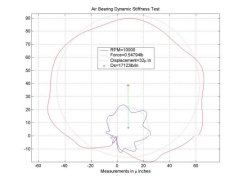
In this paper we measure three quantities to characterize the deviation of an air bearing from the idealization. The first quantity is dynamic stiffness, which measures how well the bearing resists radial shifts in the rotor axis due to the centrifugal force created by an imbalance in the rotating spindle. The second quantity is asynchronous error motion (AEM), which measures radial movement of the rotor axis that is not synchronized with the spindle rotation. The third quantity is the rotational velocity modulation or how much the RPM varies around the desired RPM value. These are the primary performance characteristics and in this paper we measure how they change with bearing RPM. In addition, we also keep track of some secondary variables which do not measure the bearing performance explicitly, but do give an indication of overall system performance; the system being composed of the air bearing, air supply, motor, encoder, controller, and amplifier. These secondary variables are the air flow into the bearing and the current through the motor windings and they help indicate problems and inconsistencies in the setup.
One popular air bearing application is hard drive head and gimbal assembly (HGA) testing. During HGA testing, a stack of disks is mounted onto an air bearing spindle and then circular tracks of data bits are written onto and read from the hard disks. Ideally the tracks should be concentric and centered and as perfectly circular as possible so that the track density does not have to be decreased to prevent the tracks from running into each other. Also, the data bits should be spaced as evenly as possible to maximize their density. The disk stack is a very representative real life load condition for an air bearing spindle. Bearings that perform well when spinning freely on their own show very significant performance drops when subjected to the forces of such a load. Even a slight imbalance in the disk stack can create large centrifugal forces on the rotor at high RPM and cause the rotor axis to shift and wobble. An air bearing's dynamic stiffness is a direct indication of how well that bearing can resist those large centrifugal forces. The AEM measurements indicate the potential eccentricity in the data tracks and the velocity modulation indicates how evenly spaced the data bits can be placed.
Dynamic Stiffness
In this paper we use the term "dynamic stiffness" to mean the quantity equal to the centrifugal force acting on the rotor in the radial direction due to an imbalance at a given axial location divided by the radial displacement of the rotor in the same axial location.

|
|
| Equation 1: Dynamic Stiffness Definition | |
The axial location is a very important parameter when characterizing the dynamic stiffness. Much of the radial displacement at a given axial location is due to rotor axis tilt as opposed to parallel axis shift. For a given amount of tilt, the magnitude of the radial displacement increases as you move away from the tilt fulcrum point. In addition, for a given amount of centrifugal force, the moment on the rotor increases the farther the force acts from the center of the bearing. So for any bearing, the dynamic stiffness measurement will be larger at an axial location closer to the fulcrum point of the bearing than it will be at an axial location that is further away.
The dynamic stiffness is not the same as the stiffness of the air film in the bearing. The dynamic stiffness might be more properly thought of as a mechanical impedance. The dynamic stiffness is a complex number that varies with rotational frequency and is very analogous to electrical impedance, which varies with alternating voltage frequency. At zero rotational frequency, the dynamic stiffness is equal to the air film stiffness just as at zero switching frequency the electrical impedance in a circuit is equal to the electrical resistance. At non-zero rotational frequency, however, the dynamic stiffness is affected by both the inertia of the rotor and the air film damping just as at non-zero switching frequency the electrical impedance is affected by both the capacitance and inductance in the circuit. Dynamic stiffness in an air bearing is a function of rotational velocity, rotor inertia, and the air film stiffness and damping. The air film stiffness and damping are most likely variables that change with rotational velocity and radial rotor displacement as well.
|
| Equation 2 : Dynamic Stiffness Functional Relationship |
One way to predict the exact relationship between these variables is to create a dynamics model of the system and solve the equations of motion. As a first approximation we can make an oversimplified model of the system by assuming that the air film stiffness and damping remain constant and by ignoring the rotational inertia and tilting of the rotor. The model becomes a one-dimensional mass-spring-dashpot system with a sinusoidal forcing function.
|
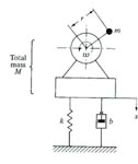
| Figure 1 : Simplified Air Bearing Spindle Dynamics Model |
The figure above is a graphical representation of the very simplified air bearing spindle system mechanical model. The total mass "M" represents the rotor mass and the imbalance mass. The imbalance mass "m" is located a distance "r" from the axis of rotation and spins at a rotational velocity equal to w. The variable "x" in the figure corresponds to an arbitrary radial direction. The centrifugal force on the rotor caused by the rotating imbalance mass acts as a sinusoidal driving force on the rotor in the x direction at a frequency equal to the rotating speed. The variables "k" and "b" are the stiffness and damping of the air film respectively. If we solve the equations of motion for this system and divide the centrifugal force by the maximum displacement, we come up with the following relationship between the system variables:
|
| Equation 3: Solutions to the Simplified Model Equations of Motion |
Note that at zero rotational frequency (w=0), SD simply equals k and the phase angle is zero. The phase angle is the phase shift of the output sinusoid with respect to the input sinusoid. When the phase angle is zero, the maximum positive displacement occurs when the input force is in the same direction as the displacement. When the phase angle is 180 degrees, the maximum positive displacement occurs when the input force is the opposite direction as the displacement. In the figure above, the air film thickness "t" will be smallest when the mass "m" is at the very bottom of its revolution and the phase angle is zero. When the phase angle is 180 degrees, "t" will be smallest when the mass is at the very top of its revolution.
In dynamics analysis, bode diagrams are often used to represent the frequency-response characteristics of dynamic systems. The frequency-response is the steady-state response of a system to a sinusoidal input. Bode diagrams consist of two separate plots, one giving the magnitude of the response versus the frequency and the other the phase angle of the response versus frequency. The dynamic stiffness is inversely proportional to the bode magnitude plot. Another way of determining the relationship between system variables would be to directly measure the frequency-response of the system, create a set of bode plots, then back out the transfer functions from the shape of the plots.
|
| Figure 2: Example Bode Plot of the Simplified Model |
The figure above is a typical bode diagram of the simplified air bearing mechanical model. The magnitude plot is shown above the phase plot. Note that the magnitude is plotted on a log-log scale. The magnitude plot is proportional to the reciprocal of the dynamic stiffness. So the simplified model predicts that for low RPM the air bearing dynamic stiffness will remain constant and the phase shift will remain zero. It then predicts that the dynamic stiffness will undergo a short drop as the phase angle begins to change, then increase indefinitely as the RPM rises. If we knew the exact proportions of the plot, we could estimate values for "M", "b", and "k".
The simplified one-dimensional mass-spring-dashpot model is most likely too simplified to predict any real trends in an air bearing. Another thing to keep in mind is that the simplified model considers movement of the rotor with respect to the stator. Often the real concern is how the rotor moves with respect to some other reference point, such as a capacitance measurement probe or write head that is attached to some support structure. Since no support structure is perfectly rigid, a better model would need to take into account the transfer function that describes the motion relationship between the stator and the real reference point. The lack of perfect rigidity in the support structure makes analysis and testing more difficult, but does allow for the interesting possibility of custom designing the support structure to tune the transfer function between the rotor and the external reference point to better meet the designers needs. Instead of simply trying to make the structure as rigid is possible, the designer might be able to tune it to minimize motion between rotor and reference point or to shift natural frequencies in the system.
Knowing the details of the relationship between the system variables, whether the relationship was found theoretically, experimentally, or by a combination of the two methods, would be very useful for predicting how the bearing would react under a set of operating conditions. A detailed bode plot or set of transfer functions would indicate resonant modes in the bearing and stability issues so the designer of an air bearing system could work around them. In this paper we make the first step in the frequency-response characterization of an air bearing by measuring the dynamic stiffness across a range of rotational speeds.