|
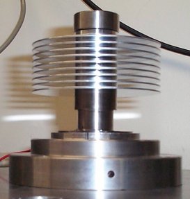
| Figure 3 : Disk Stack |
Asynchronous Error Motion (AEM)
Asynchronous error motion is movement of the rotational axis that does not occur at frequencies that are multiples of the rotational frequency. While the source of the error motions may be well defined and repetitive, they appear random relative to time, or they repeat at a frequency that is not a multiple of the rotational frequency. (Lion Precision Advanced Spindle Error Analyzer Version 7 Instruction Manual page 51). AEM can be caused by any number of disturbing forces acting on the rotor. Similar to the dynamic stiffness, much of the AEM in the rotational axis is tilt, so the farther the measurements are made from the tilt axis, the larger the motion magnitude. NRR or non-repeatable runout refers to the same type of motion. AEM is often measured both axially and radially and the radial measurements can either be from a fixed direction or one that rotates with the spindle. For the purposes of this paper we are most concerned with fixed radial AEM and when we use the term AEM this is what we imply.
Most air bearings easily measure less than one micro-inch AEM under relatively controlled conditions, with no load, and when the measurement is made close to the end of the bearing. The motion magnitude increases significantly, though, when a load is placed on the bearing and the measurements are taken at an axial location where activity normally occurs. Since the numbers are on such a small scale, even minor-seeming environmental disturbances can increase the motion dramatically. The vibrations from an air compressor running on the roof of a building can double the AEM of an air bearing spinning within that building. The first step to reducing AEM is to reduce the disturbing forces on and within the system. Vibration isolators on massive system foundations are often used to try to minimize the effects of outside disturbances.
The air bearing load itself can be a source of disturbing forces acting on the rotor. For example, a stack of disks in the HGA testing application imparts random forces in many directions on the rotor as it spins around. The disks in the stack are separated by layers of air. When the disks spin around at high speed, packets of air are ejected creating low pressure voids in the gaps between the disks. These voids are continually replenished by the surrounding air to fuel further packet loss. The effect is similar to tiny rocket blasts going off in the disk stack pushing on the rotor. These little pushes can create enormous AEM in the spindle.
|
|
| Figure 3 : Disk Stack |
The picture above shows a typical disk stack that might be used in an HGA testing application. Seagull has developed a way to minimize the random air packet loss ("puffing" as we refer to it) from the disk stack as it is spinning around by inserting "fingers" in between the disks that comb off the layers of air. (Patent Number 6,097,568).

|
| Figure 4 : Disk Stack with Fingers |
The picture above shows the fingers inserted into the disk stack to comb off the air layers before they have a chance to exhibit the puffing phenomenon. In previous tests we have seen very significant AEM reduction in a disk stack when using the fingers and in this paper we subject them to more formal tests and compare the finger effects on a variety of bearings.
Velocity Modulation
The third performance quantity that we measure in this paper is the velocity modulation of the bearing as it is spinning. The velocity of the bearing is controlled by a negative feedback loop. The controller in the system senses the velocity of the rotor from the encoder signal, compares it to the desired velocity, calculates a torque response, and sends that information to the amplifier as a current command. The amplifier sends current through the motor windings based on the current command in its own little negative feedback loop and the motor applies torque to the rotor.
|
| Figure 5 : Air Bearing Spindle System Feedback Loop |
The figure above is a block diagram of the system. In order to improve the actual velocity of the bearing, you need to both optimize the design of the feedback loop (and the individual system components) and reduce the disturbance torque acting on the bearing.
Disturbance torque on the bearing can come directly from the bearing load. The same puffing phenomenon in a disk stack that affects the AEM also acts as a source of input forces on the bearing that fight the controller's goal of maintaining constant velocity. The packets of air that continually move in and out of the disk stack and air layer system vary the momentum of the load, in effect acting as disturbance torques on the bearing rotor. The disturbance torques combine with the motor torque output to accelerate and decelerate the rotor. Unless the controller can sense the changes in velocity quickly enough to help reduce them, the bearing will speed up and slow down, speed up and slow down, and the velocity will fluctuate randomly around the desired value. The fingers placed in between the disks to stop the puffing phenomenon helps to reduce the velocity modulation of the bearing as well.
There are several ways in which the velocity modulation might be defined and measured. It is often expressed as a percentage of variation about the desired value. For example you might see a performance specification of 0.001% velocity error. One issue with expressing the error as a percentage is that for a given amount of fluctuation the percent error changes with the magnitude of the desired value. A percent velocity error at 10,000 RPM for example may not be straightforwardly comparable to a percent velocity error found at 20,000 RPM. If the variation remained constant at +/- 1 RPM say, then the percent error measurement will be twice as large at 10,000 RPM than at 20,000 RPM.
The time scale of the test is also an important variable in velocity modulation measurements. The velocity variation measured with a high sample rate over a very short period of time might be very different than the variation measured with a low sample rate over a long time period. Depending on the update frequency of the controller and the input frequency of the disturbance forces, the two measurements might be quite independent of each other. The spindle could be speeding up and slowing down at very high frequency, but the average velocity could seem very constant if it was examined infrequently over a long period of time. Conversely the spindle could be going through long cycles of slowly picking up speed, then slowly slowing down, which would not be noticed if the velocity was examined only for a short burst.
In an attempt to reconcile these issues with the velocity modulation measurements, we examine the spindle velocity on both a short-term time scale and a long-term time scale. On the short-term scale we measure intra-revolution velocity error using the individual encoder pulses over a relatively short sample time. On the long-term scale we measure inter-revolution velocity error using only the encoder index pulse over a relatively long sample time. In addition, instead of taking data over a given amount of time, we take it over a given number of spindle rotations, so that the data will be more comparable across a range of rotational velocities.
Another issue complicating the velocity error is frequency modulation of the encoder feedback signal. Encoders output a digital pulse stream at a frequency proportional to the rotational speed. A popular type of encoder is the incremental optical encoder, which consists of a rotating disk, a light source, and a photodetector (light sensor). The disk, which is mounted on the rotating shaft, has coded patterns of opaque and transparent sectors. As the disk rotates, these patterns interrupt the light emitted onto the photodetector, generating a digital or pulse signal output.

|
| Figure 6 : Optical Encoder |
Figure 6 shows the basic principle of an optical encoder. If the shaft rotates at a constant angular velocity, the markings on the disk pass by the light stream at a constant rate. The encoder outputs the digital pulse signal at the rate that the markings pass by the light stream. The controller then measures the frequency of the signal and calculates the angular velocity, knowing how many marks are on the disk. A problem arises, though, when the encoder disk is not perfectly centered on the shaft. When the disk is not centered, some of the markings are farther from the center of the shaft than they are supposed to be and some are closer. For a given shaft rotational velocity, the markings that are too far away will pass by the light stream at a higher rate than the markings that are too close. The result is that the frequency of the encoder output signal is no longer constant, but modulates around the mean frequency. The off-center encoder disk causes the output signal to vary sinusoidally.
The sinusoidal frequency modulation in the encoder output creates several problems. The encoder introduces error in the feedback signal. A very tight control loop will cause the bearing to track the incorrect feedback signal, introducing a physical velocity modulation that matches the error signal modulation. Even if a control loop is loose enough to be effectively blind to the feedback error, the error still needs to be taken into account when using the encoder output for velocity modulation testing. It can be tough, though, to separate the true velocity error from the encoder signal error.
As a solution to the encoder frequency modulation problem, Seagull has developed a special low modulation encoder with an adjustable encoder disk. With a centered disk, the encoder no longer introduces the sinusoidal error into the feedback signal and the frequency modulation is reduced. This allows for a much more accurate velocity measurement that can be used by the controller for tighter tracking or by a tester for measuring more accurate performance parameters.
Error motion in the spindle and masking errors on the encoder disk also introduce errors in the encoder output. Since the encoder disk is connected rigidly to the rotor, it feels the effects of both synchronous and asynchronous error motion of the rotor. This motion corrupts the encoder output signal just as the eccentricity of the encoder disk does. Again, since most of the error motion is rotor axis tilt, it is very important that the encoder disk is located axially as close as possible to the center of the bearing to minimize this corruption. Even if the encoder disk is perfectly centered and undergoes no unwanted error motion, though, slight variations in the transparent and opaque sectors of the encoder mask can still introduce error in the encoder output signal. It is important for the photodetector to average the signal over several of the mask sectors to minimize the effects of their variations or potential contamination. Some encoders average over more sectors than others. Seagull's new low modulation encoders average over 9 sectors while the old Seagull encoders only average over 5.
Test Equipment
Air Bearing Spindles
Seagull:
2 Hi-Capacity Biconics (biconic geometry)
2 Standard Biconics (biconic geometry)
Competitors:
2 Brand A (bispheric geometry)
2 Brand D (planar cylindrical geometry)
Controller
Seagull P2 Controller for all bearings except for Brand A.
(Brand A bearings use a 512 count encoder not compatible with the
P2 controller)
Measurement Hardware
Lion Precision Spindle Error Analyzer:
Capacitance
Probe C4-D
Capacitance Probe Driver DMT-22
Data Acquisition:
National Instruments Data Acquisition
board PCI-MIO-16E-1
Modulation Domain Analyzer:
Hewlett Packard
53310A
Software
National Instruments Labview 6.0.2
Mathworks Matlab 6.1.0
Lion Spindle Error Analyzer 7.1.0
Accessories
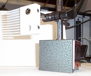
Stiffness Adapters:
|
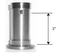
| Figure 7 : Stiffness Adapter |
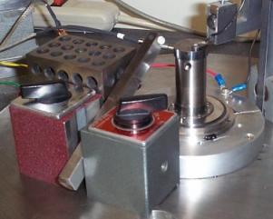
Disk Stack Adapters:
|
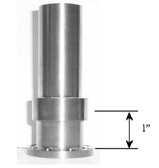
| Figure 8 : Disk Stack Adapter |
Disks and Spacers:
9 Aluminum Hard Drive Disks 95mm Diameter x 1 mm thick
8 Disk Spacers 3mm thick
Fingers:
|
| Figure 9 : Fingers |
Test Methodology
Dynamic Stiffness Measurements
The concept behind the dynamic stiffness measurements is relatively straightforward. In order to determine how much force it takes to displace the rotor axis, we simply introduce a known centrifugal force on the rotor and measure how far the rotor axis shifts off-center.
We introduce the centrifugal force on the rotor by imbalancing it.

|
| Equation 4 : Centrifugal Force Due to Rotating Imbalance |
The centrifugal force on the rotor is equal to the imbalance on the rotor times the rotational velocity w squared. The imbalance is equal to the mass of the imbalance "m" times the distance "r" the imbalance is located from the axis of rotation. The dimensions of the imbalance are mass-length and the dimensions of w are angle/time. The centrifugal force on the rotor is linearly proportional to the imbalance magnitude. If we double the imbalance in the rotor by either adding more mass or by moving the mass farther from the axis of rotation, the centrifugal force also doubles. The centrifugal force, however, grows geometrically with the rotational velocity. If we double the angular velocity of the rotor, the centrifugal force quadruples. So even small imbalances can create quite large forces on the rotor at high RPM.
We use the stiffness adapter to apply the imbalance to the rotor for the stiffness tests. The adapter bolts onto the end of the rotor and has a setscrew hole drilled through it radially. As mentioned in the background, the axial location is a very important variable when measuring and specifying the dynamic stiffness. We chose to use an axial location 2 inches from the top of the bolt heads holding the adapter onto the rotor, since this is a typical load location for many air bearing spindle applications. The setscrew can be moved radially to change the amount of imbalance in the adapter. The setscrews in the adapters (we need a different adapter for every incompatible bolt hole pattern in the bearings) have mass of around 2.5 grams. The setscrews can be moved as far as 0.18 inches from their balanced positions, so we can introduce as much as 0.45 gram-inches of imbalance (mixing English and metric units). It would not be difficult to have this much imbalance in a haphazardly placed hard drive disk stack in an HGA tester. At 30,000 RPM that relatively small amount of imbalance applies over 25 lbs of force on the rotor, so it is very important that the bearing is stiff enough to resist those high forces if you want to run at high speed. One approximation we make is that the imbalance remains constant during the tests, even though it changes slightly with the rotor axis displacement. We ignore this change, though, since it is several orders of magnitude less than the initial imbalance distance from the axis of rotation.
So after we have introduced a known amount of imbalance into the rotor, the next step is to measure how far that imbalance displaces the rotor axis as the rotor spins at speed. We find the location of the rotor axis by examining the runout of the adapter with a non-contact capacitance probe. The probe measures the distance between the probe tip and the side of the adapter.
|
| Figure 10: Dynamic Stiffness Test Setup |
The picture above shows a typical setup for the dynamic stiffness tests. Note that because the setscrew hole punctures both sides of the adapter, the probe cannot be placed at the exact same axial location as the imbalance because the holes would interfere with the runout measurements. So we chose to place the probe at a slightly greater axial distance from the center of the bearing than the imbalance. This makes all of the stiffness measurements slightly lower than they would be if the probe measured the same location as the imbalance. We made sure to keep this distance the same on all of the bearings, though, so the results could be compared properly. The Lion Precision capacitance probes can be used in two ranges: HI and LO. The HI range measures at a higher resolution over a shorter distance, while the LO range measures a lower resolution over a larger distance. We use the Lion Precision capacitance probes in LO range for the dynamic stiffness tests to give ourselves plenty of space between the probe tip and the adapter. We do not want the adapter to hit the probe when the runout is large.
To measure the runout of the adapter and compute the location of the rotor axis, we wrote several programs in Labview and Matlab to do the data acquisition and manipulation. The Labview data acquisition program first finds the rotational velocity from the encoder, then determines the sample rate necessary to measure the runout in 40 locations around the circumference of the adapter. We chose 40 samples per revolution because that was the maximum number that could be taken by the data acquisition card while the spindle was spinning at 30,000 RPM. The program then waits until it sees the index pulse from the encoder, then takes the 40 runout measurements and stores them into an array. It does this for 20 revolutions, so afterwards it has 20 runout measurements at each of the 40 circumferential locations around the adapter. The Labview program then sends this information to the Matlab program. The Matlab program takes the median value of the 20 samples at each of the 40 locations and calls that the runout for that spot. (We make multiple measurements at each point to minimize the corrupting effects that the AEM and the velocity modulation have on the tests.) So now the program has 40 runout measurements equally spaced around the circumference of the adapter. It then scales the data by subtracting the smallest runout measurement from all of the runout measurements. The smallest runout measurement is the smallest gap size from the probe to the adapter, which is not necessarily constant between bearings. So after all that we are left with 40 scaled runout measurements equally spaced around the circumference of the adapter, with the first measurement corresponding to the index pulse.
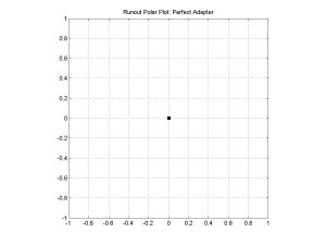
A perfectly balanced, perfectly cylindrical, perfectly centered adapter would leave the programs above with 40 scaled runout measurements all equal to zero. If we plotted these data in polar coordinates, we would simply see a single point at the origin.
|
| Figure 11 : Runout Polar Plot for a Perfect Adapter |
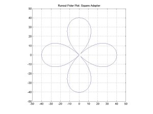
The runout polar plot for the perfect adapter is not very exciting. All of the points are on the origin. If the cross-section of the adapter was square shaped, however, instead of circular, but still perfectly balanced and centered, the runout polar plot would look a little more interesting.
|
| Figure 12 : Runout Polar Plot for a Square Adapter |
The four points at the origin of the runout polar plot with the square adapter correspond to the four corners of the square. Not all of the points are on the origin this time, but the plot is still centered about the origin. Now if we take the square adapter and simply move it off center from the axis of rotation of the bearing, the runout polar plot changes again.
|
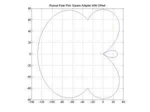
| Figure 13 : Runout Polar Plot of a Square Adapter with Offset |
The plot above shows the runout polar plot of a square adapter with an offset of magnitude 50. Now the plot is no longer centered about the origin. To find the approximate center of the data, we can do a least squares circle fit to the data and find the location of the center of the best-fit circle. If we do least squares circle fits on both of the runout polar plots and take the difference between the two centers of the circles, we can, in effect, measure the offset of the adapter.
|
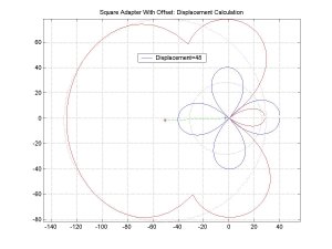
| Figure 14 : Offset Measurement for the Square Adapter |
The barely visible circular dotted lines in the plot above are the best-fit circles to the two data sets. The centers of both of the best-fit circles are shown on the plot along with a line that connects them. The length of that connecting line is approximately the magnitude of the adapter offset. In this simulation, the offset of 50 was measured as 48.
We use the same technique for measuring the displacement of the rotor axis during the dynamic stiffness tests. In the tests we use a cylindrical adapter, centered with a dial indicator, and take runout measurements on it both when it is balanced and when it is unbalanced. The difference between the centers of both data sets is the displacement of the rotor axis of the bearing due to the centrifugal force caused by the imbalance.

|
| Figure 15 : Typical Dynamic Stiffness Measurement Polar Plot |
The figure above shows a typical dynamic stiffness measurement for a spindle running at 10,000 RPM. The small data set and best-fit circle are the runout measurements when the adapter was balanced. As you can see on the plot, the adapter is not perfectly round, nor perfectly centered, otherwise all of the points would be on the origin. If the adapter was perfectly round and centered, then we would not need to take the initial balanced runout measurements every time, we could simply assume the initial adapter center was at the origin. Taking the initial measurements improves the accuracy of the tests in light of the imperfect conditions. The large data set and best-fit circle correspond to the runout on the adapter when it is unbalanced. The center of the adapter did not change with respect to the center of the rotor, rather the rotor axis shifts with respect to the axis of rotation. The program calculates the centrifugal force on the rotor knowing the imbalance magnitude and the rotational velocity, then divides the force by the rotor axis displacement to find the dynamic stiffness.
In addition to finding the distance between the centers of the data sets, we might also find the direction. The direction of the rotor axis shift corresponds to the phase angle. If we knew the location of the imbalance with respect to the index pulse of the encoder, plus we knew of all the time delays in the data acquisition system, we could use the direction information to map the phase angle across a range of bearing speeds to get the second half of the bode plot of the frequency response for the system. We noticed, by matching polar runout plots with physical markings on the adapters, that there is indeed a significant time delay from the index pulse signal to the time it takes the data acquisition system to take the first measurement. This means that the zero degree angle does not necessarily match up with the index pulse. For example if there was a 1 ms time delay in the data acquisition system, then at 20,000 RPM (3 ms/rotation), the bearing will have spun 1/3 of a rotation between the time the encoder output the index pulse and the time the software was able take the first runout measurement with the probe. The software continues to take the forty measurements, so it measures over an entire revolution of the spindle, but the first measurement does not exactly coincide with the index pulse. With a constant time delay, the angle between the index pulse and the first measurement will change with RPM. We found this to indeed be the case. This angle change would make a phase angle calculation more difficult, but does not necessarily corrupt the dynamic stiffness measurements. It is another reason, though, why we need to take initial runout measurements of the adapter while it is balanced at every RPM increment, before we take the imbalanced runout measurements at the same RPM increments.
Another assumption we make with these dynamic stiffness measurements is that the dynamic stiffness does not change with radial direction. We arbitrarily choose a radial location when we place the probe. It is possible for the dynamic stiffness to be slightly direction dependent, though. For example a slightly out of round stator might affect the air film properties creating changes in the dynamic stiffness. Along these same lines, we also assume that the air properties remain constant between the capacitance probe and the adapter. An out of round adapter may create air flow patterns that change the air capacitance and slightly corrupt the capacitance probe readings, but we assume these effects are negligible.